Nearly Every JPEG on Earth Runs on Math a Reviewer Called Too Simple to Fund in 1972

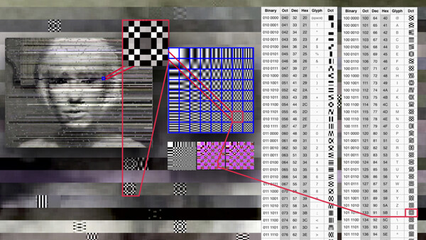
In early 1972, a Kansas State University professor named Nasir Ahmed sent the National Science Foundation a proposal to study a cosine transform built out of Chebyshev polynomials. NSF declined to fund it, and in his own written account of what happened, Ahmed recalled one reviewer's comment coming down to the whole idea seeming "too simple." That idea is the arithmetic sitting underneath essentially every JPEG in your catalog.

The Summer That Produced the Transform

Ahmed taught at Kansas State from 1968 to 1983, and he arrived in the middle of a noisy period in image coding. Researchers were introducing new orthogonal transforms faster than anyone could evaluate them, and the comparisons were often qualitative, made by looking at a set of standard test images that had been squeezed and reconstructed. Groups at the University of Southern California's Image Processing Institute and at UCLA pushed the field toward real measurement, and the Karhunen-Loeve transform became the yardstick, because under a first-order Markov model of an image, it is provably the best you can do for mean-square error.

The Karhunen-Loeve transform had one crippling problem. It depends on the statistics of the specific data you feed it, so there was no fast, fixed algorithm to compute it. Ahmed went looking for a stand-in: a signal-independent transform that behaved almost as well but could be computed quickly on any block of pixels. He found his lead in a 1968 Prentice-Hall textbook on evaluating mathematical functions by computer, in two sections on Chebyshev interpolation. Cosine functions of that family, it turned out, look remarkably like the Karhunen-Loeve basis functions across exactly the range of pixel-to-pixel correlation that real photographs occupy.

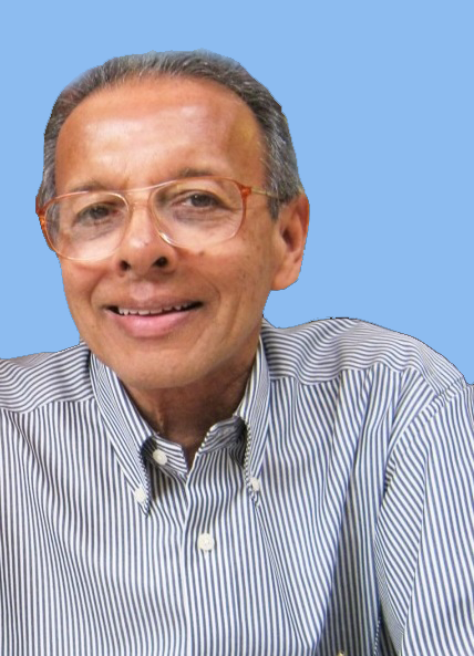
That was the proposal NSF turned down. Ahmed described the episode to IEEE Spectrum years later: "I had a strong intuition that I could find an efficient way to compress digital signal data. But to my surprise, the reviewers said the idea was too simple, so they rejected the proposal."

He did the work anyway, without the grant. His 1991 recollection in the journal Digital Signal Processing is blunt about the disappointment and specific about what followed: he took the problem to his doctoral student T. Natarajan and to his friend K. R. Rao at the University of Texas at Arlington, and he remembered dedicating the whole summer of 1973 to it. The numbers came back better than he trusted. "The results that we got appeared too good to be true," he wrote, so he took them to Harry Andrews of the USC group at a conference in New Orleans, where both were speaking at a session on Walsh functions. Andrews mailed him a program to score the transform against the rate-distortion criterion, the tougher quantitative test of the day. It held up, landing close to the Karhunen-Loeve ceiling and ahead of everything else on the table. Andrews told him to publish.

Ahmed, Natarajan, and Rao sent the paper to IEEE Transactions on Computers, where it ran in the January 1974 issue across four pages, 90 through 93. They filed it as a correspondence item rather than a full paper, for the unglamorous reason that correspondence got into print faster.

What the Transform Does to an 8x8 Block

Open a typical color JPEG, and the encoder that made it did the same thing to your picture. It converted the image to a brightness channel plus two color channels, then sliced each channel into tiles eight pixels on a side. Grayscale files carry one channel and CMYK files four, but the tiling and everything after it work the same way. Each tile is 64 numbers. Before anything else, the encoder subtracts 128 from every 8-bit sample so the values sit between -128 and 127, centered on zero.

Then comes the discrete cosine transform, run in two dimensions across the tile. Sixty-four numbers go in and 64 numbers come out, and the output numbers are not pixels. Each one is the weight of a fixed pattern. The first pattern is flat, a uniform gray. The next few are gentle gradients, light on one side and dark on the other. They get busier as you move down and to the right, ending in a checkerboard so fine that adjacent pixels alternate. Multiply all 64 patterns by their weights, add them up, and the original tile comes back.

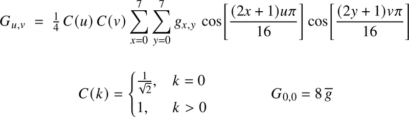
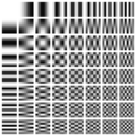
The top-left number is the DC coefficient, and it is exactly eight times the average value of the level-shifted tile. Everything else is called an AC coefficient, and each describes how much detail of a particular fineness and direction the tile contains. Real photographs are mostly smooth at this scale. Skin, sky, a defocused background, the shadow side of a face: those tiles put nearly all of their energy into the top-left corner and leave the fine patterns close to zero. That concentration is the whole point, and it is what Ahmed's rate-distortion tests were measuring.

Nothing has been thrown away yet. The transform is reversible down to rounding error. The 8x8 tile size is not Ahmed's either. His paper defines the transform for a sequence of any length; eight was a standards-era decision, and the two efforts that settled on it were running in parallel rather than one trailing the other. The JPEG committee selected the 8x8 adaptive DCT proposal at Copenhagen in January 1988, and H.261 was approved that November carrying the same 8x8 block. Eight was small enough to compute cheaply on 1980s hardware and large enough to be worth doing.

The Quality Slider Is a Table of Divisors

The loss happens in the next step. Each of the 64 coefficients gets divided by its own number from an 8x8 quantization table, and the result is rounded to a whole number. Annex K of the JPEG specification publishes example tables derived from psychovisual experiments, and libjpeg, the Independent JPEG Group implementation that a great deal of photo software still descends from, ships them as its base tables. The luminance table starts at 16 in the top-left corner and ends at 99 in the bottom-right. Your eye tolerates far more error in fine texture than in overall brightness, and the table is shaped to exploit that.

Your quality slider scales that table, and the math is simple enough to do in your head. At quality 50 in libjpeg, the table is used exactly as printed. Above 50, the scaling percentage is 200 minus twice the quality; below 50, it is 5,000 divided by the quality. Push those through, and the divisors become concrete. At quality 90, the top-left coefficient is divided by 3 and the bottom-right by 20. At quality 50, by 16 and 99. At quality 10, by 80 and 495, or by 255 if the encoder is forcing baseline-compatible tables.

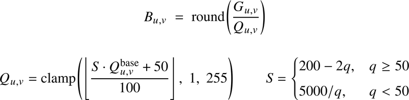
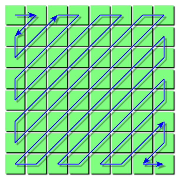
Take a coefficient worth 40 and divide it by 99. It rounds to zero. In a smooth tile, most of the high-frequency coefficients round to zero at ordinary quality settings, and the encoder then reads the tile out in a zigzag from the lowest frequency to the highest so all those zeros bunch together at the end, where run-length and Huffman coding crush them into almost nothing. Your file gets small because you deleted the checkerboards.

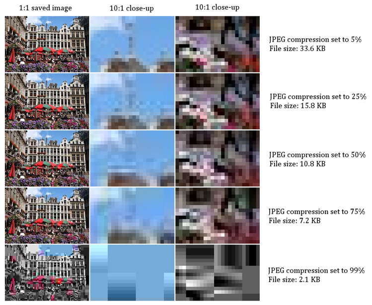
The failure modes follow directly. When the divisors get coarse, neighboring tiles reconstruct to slightly different averages and the eight-pixel grid becomes visible, which is why an over-compressed sky bands into squares instead of banding smoothly. Hard edges pick up a faint halo, because a sharp step needs the fine patterns to reproduce and you just zeroed them. Fine red lettering smears worse than fine black lettering, because the color channels get the harsher table and, in libjpeg's default configuration, are also stored at half resolution horizontally and vertically before the transform ever runs.

The Discrete Cosine Transform Has an Author

The discrete cosine transform is usually described as though it were weather: a fact of mathematics that was always sitting there, unowned and unauthored, waiting for engineers to pick it up. Fourier analysis is old, Chebyshev polynomials are old, and cosine functions belong to nobody.

The record is more specific than that. What Ahmed proposed in 1972 was not cosines in general but a particular discrete transform, offered as a computable substitute for the Karhunen-Loeve transform in image coding, and then demonstrated to be one on two different quantitative criteria. It has an author, a rejection, a named doctoral student, a collaborator in Arlington, a colleague at USC who lent out his test program, and a publication date. The choice to route it into a journal, deliberately in the format that would print fastest, put it into the open technical literature rather than into a portfolio. Ahmed closed his 1991 note by saying it was "indeed gratifying" to see the transform become essentially a standard in image compression, which is the language of an author watching his work get used rather than licensed. When the JPEG committee began its work in 1986, the transform at the center of the new standard was already published mathematics that anyone could implement.

Recognition came slowly. Ahmed moved to the University of New Mexico in 1983 and spent the rest of his career there, taking one of the university's twelve Presidential Professorships in 1985, chairing the electrical and computer engineering department, and serving as interim dean of engineering. Outside the field, almost nobody knew his name until 2021, when NBC's "This Is Us" dramatized his work in a February episode, at a moment when its whole audience was living on video calls. In 2026, the National Academy of Engineering elected him a member, and IEEE gave him its Fourier Award for Signal Processing, with a citation crediting his contributions to the digital revolution through developing the discrete cosine transform. That is 54 years after the proposal was judged too simple to fund.

How to Export With This in Mind

Quality 100 is not lossless, and treating it as though it were costs you nothing but storage space and a false sense of safety. At libjpeg quality 100, the scaling factor hits zero, every divisor in the table becomes 1, and that is the floor of quantization rather than the absence of it. The transform itself still rounds. Chroma subsampling, which is a separate setting from the quality slider, may still be throwing away three quarters of your color resolution. If you need a genuinely lossless intermediate, JPEG's own lossless mode is a different algorithm that does not use the transform at all and is supported almost nowhere; use a PSD, or a TIFF or DNG written with lossless compression, instead.

Quality numbers do not travel between programs. Photoshop's 0-to-12 scale uses its own quantization tables, camera manufacturers use theirs, and libjpeg-derived exporters use the Annex K tables scaled by the formula above. A file saved at 80 in one application is not the same file as one saved at 80 in another, so judge exports by looking at the output at 100 percent rather than by matching numbers across apps. If you want to work through the export panel systematically, Fstoppers' introduction to Adobe Lightroom covers the settings that actually change the file.

Every save is a fresh divide-and-round. Open a JPEG, adjust exposure, save it again, and the encoder quantizes coefficients that were already quantized, on a grid that may no longer align with the first pass if you cropped. Keep the raw file or a lossless master, do your editing there, and export a JPEG once, at the size you actually need. Exporting a 45-megapixel frame at quality 95 for a website is the opposite of careful; downsizing first and exporting at 80 usually produces a smaller file that looks better, because resampling removes the fine detail that would have been quantized into blocking artifacts anyway.

The formats that took over from JPEG kept the transform instead of replacing it. HEVC, which is what your iPhone's HEIC files use, runs integer approximations of the same transform at sizes from 4x4 up to 32x32, with a sine-based variant reserved for the smallest intra-predicted luma blocks. JPEG XL's VarDCT mode uses variable-size DCT blocks running from 2x2 to 256x256. Wavelet-based JPEG 2000 went the other way and never displaced JPEG for general use. Fifty-four years on from the rejection, the newest image formats are still mostly arguing about how big the block should be.

Lead image by Rosa Menkman, CC BY 2.0. Source.